¶ Overview
This page provides an overview of how to tune a PID for a shooter.
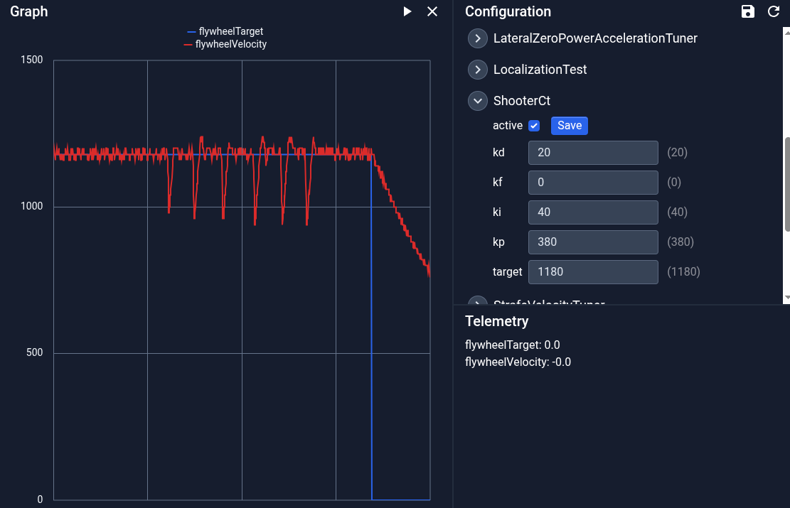
Below are a few graphs showcasing different situations that you might encounter.
The process we use for flywheels is as follows:
- Start with all coefficients at 0
- Raise
Kfuntil the motor starts moving on its own, then back it off just below the threshold point. This parameter compensates static friction and stiction. For a relatively frictionless flywheel, this is 0. - Raise
Kpuntil the system correctly follows the target in desired time. Oscillations are acceptable. - Raise
Kd(small values) until oscillations are compensated for and the system is not too damped. - If the system suffers from steady-state error, Raise
Kiuntil the error dissapears in a time equivalent with twice the settling time with onlyKpandKd. Keeping this value low can help avoid systematic instability.
The result of this procedure is often an overcompensated PID. If the system does not tolerate aggressiveness well, back off all values by about 15-30%.
Systems with higher inertia (mass) can tolerate too high Kd values. Low-inertia and overlapped control values can cause unwanted vibrations at high frequencies.
The tests are done using a 4200 RPM motor attached to a AndyMark 4inch 30A compliant wheel.
| Undercompensated Kp | Undercompensated Ki (steady state error) |
|---|---|
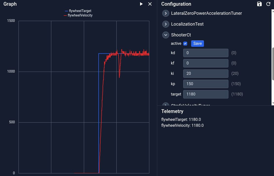 |
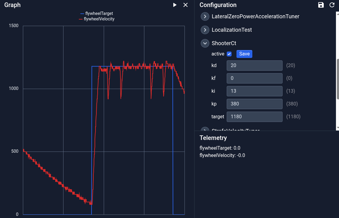 |
| Better Ki but not enough | Ki, Kd induced oscillations |
|---|---|
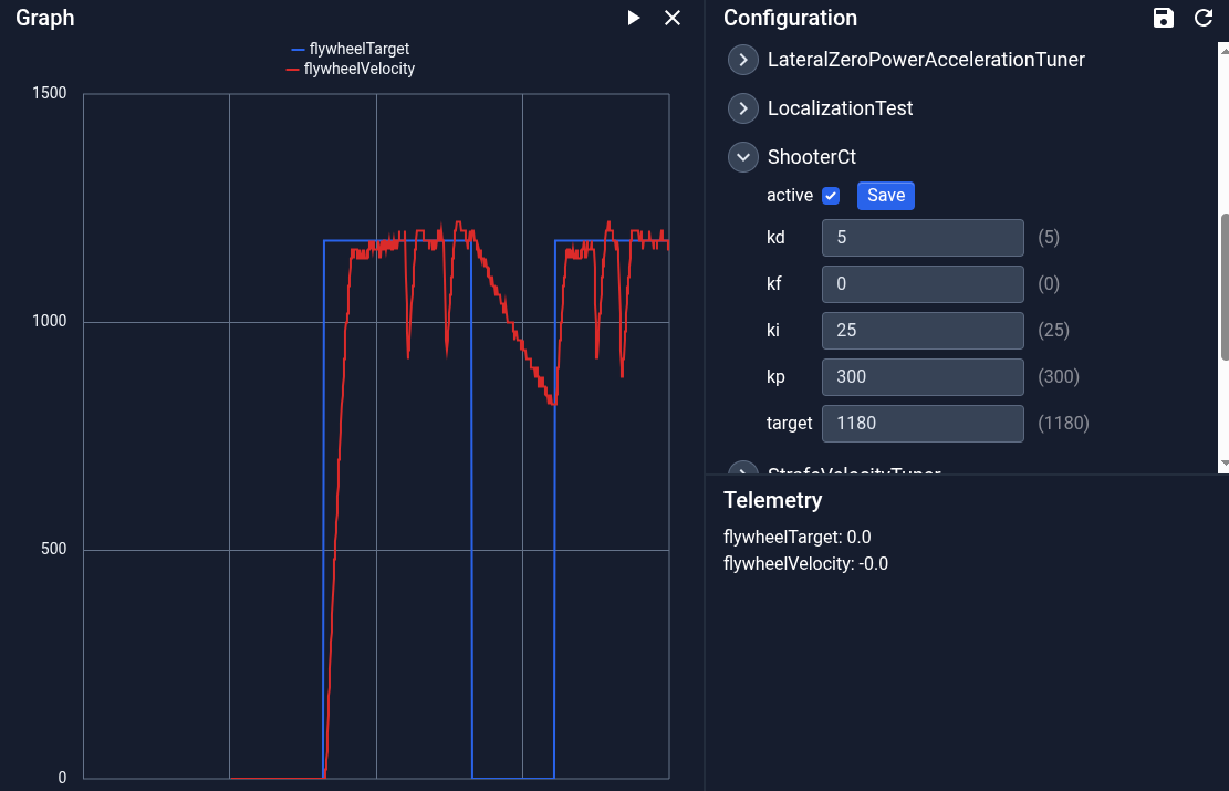 |
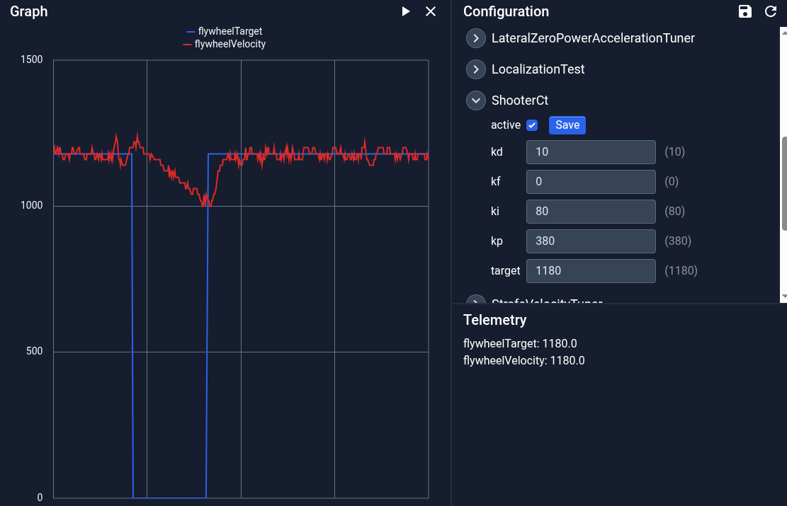 |
| Almost Perfect |
|---|
 |
¶ Motor analytical performance
SI unit conversions:
- No-load speed: 6000 RPM → ω₀ = 6000 × 2π/60 = 628.3 rad/s
- Stall torque: 1.47 kg·cm → τ_stall = 1.47 × 0.01 × 9.81 = 0.1442 N·m
- Stall current: I_stall = 9.2 A
- No-load current: I₀ = 0.25 A
- Voltage: V = 12 V
Brushed DC motor linear model:
Brushed DC Motor model: V = R·I + K_e·ω, so:
- Terminal resistance: R = V / I_stall = 12 / 9.2 = 1.304 Ω
- Back-EMF constant: K_e = V / ω₀ = 12 / 628.3 = 0.01910 V·s/rad
- Torque constant: K_t = τ_stall / I_stall = 0.1442 / 9.2 = 0.01567 N·m/A
(K_e ≈ K_t as expected for an ideal DC motor)
The no-load current (0.25 A) accounts for friction torque:
The generalized equations for any voltage V and angular speed ω, with a number of N motors in parallel:
| Parameter | Symbol | Value | Unit |
|---|---|---|---|
| Terminal resistance | R | 1.304 | Ω |
| Back-EMF constant | Kₑ | 0.01910 | V·s/rad |
| Torque constant | Kₜ | 0.01567 | N·m/A |
| Friction torque | τ_f | 0.00392 | N·m |
| No-load speed @ 12 V | ω₀ | 628.3 | rad/s |
| Stall torque @ 12 V | τ_stall | 0.1442 | N·m |
¶ Battery performance
The circuit equation for N identical loads in parallel, each described by I(V):
The operating point is the voltage V where the source line and the aggregate load curve intersect:
To combine with motor formulation, substitute I_load with the motor's formula and solve for V.
Afterwards, substitute V in the motor torque formula and the result should be a torque(speed) relation.
¶ Gearbox with wheel formulation
Consider a motion source with angular speed w_m and torque tau_m, our gearbox reduces speed and amplifies torque by a ratio of G. The efficiency of the gearbox is eta (tipically 96%)
The output axle is attached to a wheel of diameter D. This system is translated to linear force and linear speed:
We can further combine these two formulations to transform from motor specs to linear movement (acceleration and speed):
We can transform to linear space acceleration:
¶ Putting it all together
To transform from acceleration(speed) to speed(time), use the acceleration textbook formula (dv/dt). From previous calculations, the acceleration(speed) should be first order function
This differential equation has a well known solution:
Special cases:
- If
β = 0→v(t) = v₀ · eᵅᵗ(pure exponential growth/decay) - If
α < 0→ speed decays to a terminal velocityv_terminal = -β/α - If
α = 0→ constant acceleration,v(t) = v₀ + β·t
Integrating v(t) in respect to time to get possition(time):